Summary and Discussion
Algorithm
A general purpose distributed robot formations algorithm has been presented. Robots are represented as cells in a “robot-space cellular automaton”. Connectivity of the automaton is guaranteed as it is expressed as the union of all cell neighborhoods. A human operator sends a formation definition to some cell, designating it as the seed of the automaton. It is emphasized that this cell is not a leader, but rather an initiator of the coordination process—thus, this algorithm distinguishes itself as being leaderless. Each robot cell state consists of its distance and orientation in 2-dimensional space in relation to neighboring robots. Using only local information, these robots are able to establish and maintain a variety of formations.
As described in 1-Dimensional Robot-Space Cellular Automata, the initial conception of the algorithm considered formations defined by a single mathematical function [19]. Motivated by SSP, the algorithm was generalized such that a formation could be defined by any number of mathematical functions—the goal: to produce grids. Using Equation 8 to solve for desired relationships with neighboring robots, it was discovered that oddly—but interestingly—shaped “armed structures” would emerge; this result was intuitive, as a cell’s function-relative position is used in this calculation. In order to achieve the desired lattice structures, an alternative equation—Equation 33—was developed that omitted this cell property. The result: hexagonal and square lattices (see Implementation Results in 2-Dimensional Robot-Space Cellular Automata for details).
Formation classification
Previous work [19] and observations in Formations Defined by Multiple Functions lead to a preliminary classification of formations that can be represented as robot-space cellular automata in this algorithm; further study is necessary to develop an exhaustive list, and is left as future work.
- Non-formation (swarm)—A distinction has already been made between a swarm and a formation (see Fig. 6 for an example)—the former does not assume any particular organization, while the latter requires a definite structure. Nonetheless, swarms have a place in the algorithm, likely represented by 2-dimensional cellular automata. From Equation 26, consider a situation where M = 0 and, thus, f' is an empty set. Given a formation defined in this way, it is clear that desired relationships are unable to be calculated using either of Equations 8 or 33; however, variables R and Φ in the formation definition provide enough information to demonstrate some interesting behavior. Robots still must maintain a range R to one another. This type of definition is similar to the approaches taken by [6, 25] and has the possibility of generating emergent lattice structures; however, as previously stated, this situation is less controlled and would not be a reliable method for grid organization. Robots can also use Φ to generate a common heading. McLurkin [18] utilizes the ability of swarm robots to orient to the same heading in order to follow a beacon. Note that, in any case, a neighborhood must be considered. For a generic swarm and a cell ci, its neighborhood Hi could simply be all cells in the automaton (i.e., Hi = C). Other applications may provide a specific neighborhood definition or even allow the neighborhood to be dynamically determined based on robots in proximity.
- Explicit formation—As in Class I, a formation is defined with M = 0 and f' as an empty set. However, this classification differs in that strict (explicit) relationships (and potentially neighborhoods) are provided (much like how a marching band is formed, as in Fig. 8). The dimensionality of the automaton would be based upon the configuration of neighborhoods and the relationships within them. This categorization provides opportunity for nearly any type of structure or shape imaginable, in that the formation is not restricted to be being defined by one or many mathematical functions. While a wide variety of different formations could be generated by this approach, it is likely unappealing as there is a considerable amount of overhead associated with individually specifying neighborhood relationships for each cell.
- Straight line formation—It has been observed that formations defined by single functions usually require the use of Equation 8 when determining desired relationship—this is intuitive. Recall that Equation 11 holds that, for a formation to be stable, the calculated relationships between neighbors must be equal in magnitude, but opposite in direction; if Equation 33 were used on a single-function formation, the latter of these two claims would not be true—indeed, the relationships would be equal in magnitude, however, they would not be opposite in direction. The only exception to this noted thus far is in the case of f(x) = a x (i.e., any straight line; see Fig. 22); this is due to the fact that the set left and right relationships will be the same for any formation-relative position used in the calculation of Equations 8 and 9. Thus, for formations in this category, either Equation 8 or Equation 33 can be used for purposes of calculating desired relationships. The nature of the line also suggests that this category will be represented by a 1-dimensional cellular automaton.
- Function-based formation—This classification is based on the initial definition of the formation control algorithm in 1-Dimensional Robot-Space Cellular Automata and, for this reason, is considered the simplest (represented as a 1-dimensional cellular automaton), most general (conforming to a variety of different functions), and most clearly stable (see Eq. 11 for a description of why it is stable) type of formation identified. For purposes of calculating desired relationships, Equation 8 is used.
- Branching formation—Formations in this category describe those previously referred to as “armed structures” (see Figs. 31 & 34)—the use of the “branching” descriptor comes from the notion that each “arm” is like a “limb” (or “branch”) of the formation. Multiple functions are used to define a formation (i.e., M > 1), and Equation 8 is used to calculate desired relationships. This category has the interesting result of forming neighborhoods with nonstandard sizes, as a cell with a formation-relative position on a “branch” would likely have a smaller neighborhood than that of those cells closer to the seed. For this reason, these neighborhoods must be formed dynamically to alleviate the overhead of operator-definition (see Dynamic Neighborhoods in the next section for details). Combining neighborhoods would generate a 2-dimensional cellular automaton, albeit somewhat irregular.
- Lattice formation—In 2-Dimensional Robot-Space Cellular Automata, it was shown that these types of formations form tight, interlaced grids through the use of Equation 33 for desired relationship determination. Unlike those in Class V, these types of formations have a standard neighborhood size in a 2-dimensional automaton. Potential for collisions is high, as robots will be working in proximity of one another; however, the grid still remains stable as Equation 11 still holds.
Erroneous relationships
In extreme cases of any class of formation, it is theoretically possible to calculate more than two desired relationships for a given function [Fig. 37].
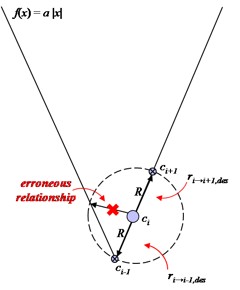 |
Fortunately, this problem is easy to alleviate. Recall that both Equations 8 and 33 solve the roots for the vector v, which are then used in Equation 9 to determine ri→j,des for all neighbors. In the case that v yields more than two solutions, one simply considers that, to maintain a sense of continuity on a function, the two values of vx nearest to the x-component of the formation-relative position pi,x of cell ci produce the proper neighbor relation. In other words, the two relationships that are valid are those that minimize the function:
Robot Platform
Hardware
A total of 19 robots were developed for the purpose of this project. These robots are homogeneous in terms of hardware—atop a two-wheeled ScooterBot II base sits an XBCv2 microcontroller with a color camera; an XBee wireless communication module with a custom interface to the XBC allows for inter-robot communication. A colored bar-coding system was used for neighbor identification, with each robot featuring a unique “face”.
The wheeled platform performed better than expected, demonstrating very accurate motion control (via back-EMF) with minimal slippage on the tile surface used for testing. robot symmetry likely balanced the effects of environmental dynamics, aiding in such positive locomotive results. The size of the robot is ideal for multi-robot systems, as it is large enough to facilitate the aforementioned hardware (with room for sensor expansion, if desired), while being small enough such that a large collection of robots can actually be tested in an average-sized room. The robots are also very sturdy, surviving a few tumbles in the lab and during travel. For these reasons, the ScooterBot base is recommended as an inexpensive and easy-to-use platform for single- and multi-robot systems.
The requirements of the formation control algorithm (in terms of motion control, data communication, and vision processing) promised to push the XBC to its limits—fortunately, the microcontroller was up to the task. Computation power and program execution time proved to be more than adequate for the purposes of this work. The color camera performed well; tracking blobs of preprogrammed color models (orange, green, and magenta) was consistent across all robots; auto white-balancing allowed for adaptation to different lighting conditions. Note that, since the XBCv2 has a serial interface, downloading programs can be rather time-consuming. An alternative would be to use the XBCv3, which is USB-based, thus, decreasing download time; however, in order to utilize wireless communication, a new interface board would have to be created.
The XBee module and PCB provided transparent serial communication between robots, which used packet addressing to propagate information within their respective neighborhoods. Acknowledgments and automatic retries implemented on the chip itself reduced the amount of packet loss. In cases where a large amount of data is being relayed, transmission time can be high, but not unreasonable. The most notable problems with serial communication resulted from its integration with software (discussed below). Given the algorithm’s high dependence on communication, the module proved to be very reliable.
Robot “faces” were the hallmark of the robot platform, as robots were able to consistently identify and localize with their neighbors—results were better than expected. Initial estimates showed that a robot would only be able to identify a neighbor if it was within a range of 18" to 24"—a rather limited threshold. However, upon testing, it was observed that robots could be identified at distances ranging from 16" to as far as 40". In switching from the previous banding method (see Neighbor localization in 1-dimensional Robot-Space Cellular Automata), the physical height of the orange band had to be reduced, leading one to believe that perceived distances might suffer; however, distances remained consistent when the “faces” were implemented. This identification system provides great opportunity for further multi-robot coordination research (see Multi-robot sandbox in Future Work for details).
Software
The formation control algorithm was implemented in an extensive collection of libraries written and tested in Interactive C. Unfortunately, the use of this language was the greatest obstacle to progress. While IC, indeed, has a large population of users nationally for testing at the middle school and high school levels, more advanced programming concepts at the collegiate research level remain untested and buggy. A vast majority of the time spent was on debugging the language itself, often necessitating undesirable workarounds (not fixes) and generating counterintuitive results.
It was discovered that, if a globally-defined character array (primarily serving the role as a communication buffer) exists with an odd number of elements and a serial command is used, that the system would freeze. Following suit, if an array is a member of some data structure, it would often crash the compiler. The built-in IC simulator had a tendency to produce results contrary to that of the hardware. For example, a programmer’s intuition says—and the simulator validates—that if a long-integer were to exceed its maximum value, it would wrap around, becoming negative; however, when such a situation occurs on the XBC, the value is instead set to its maximum. Additional unexpected problems made even documentation difficult—if a certain combination of keys (often Backspace followed by a Return) is pressed while making multiple single-line comments in succession, the compiler will crash.
The bundled serial communication library, xbcserial.ic, provides basic functionality, but would occasionally cause the XBC to lock up. Effort was made to alleviate this, with minor modifications to the library that seemed to reduce—but not eliminate—the problem. For this reason, great care was taken to handle errors that could actually be detected in Packet.ic and Communication.ic (see Robot Code). Unfortunately, undetectable errors still would cause a system deadlock. This is likely the result of high network activity on a clearly untested serial communication system.
IC also offers support for multi-threading; however, it imposes extreme undocumented limitations that forced almost the entire algorithm to be re-implemented. It was observed that when a motor command was used in one thread and serial communication in another that erratic behavior would occur, such as the calling of the last function in a random file or, more often, deadlock. This problem was circumvented (but by no means “solved”) by running the entire algorithm as single, sequential process. This drastically increased the amount of time for coordination. Robots would often pause for seconds at a time to process communicated packets while in the middle of other important operations, such as searching for neighbors or moving to correct for state errors. This would introduce a noticeable amount of error in the motion of the robot, as the dynamics of starting and stopping often introduced wheel slippage; however, the control algorithm demonstrated high fault tolerance and robustness, as robot movements would still produce the desired formation.
The worst limitation imposed by IC was that of program size, allowing only 48K of code to be transferred to the XBC (i.e., not a hardware limitation). Many of the software issues discussed required rather lengthy workarounds, reducing the amount of space available for actually implementing the algorithm itself. Preprocessor definitions were utilized to reduce the compilation of unused functions, but this was tedious and should not have been necessary. In the worst case, crucial components of the implementation had to be commented out in order to demonstrate, piecewise, certain aspects of the system.
For future implementations of the algorithm, a different language should be utilized.
Future Work
Dynamic neighborhoods
It has been shown that, as the formation changes, the neighborhood may change as well. In particular, consider a formation change in which the number of defining functions changes (for example, a straight line to a lattice). The current implementation of this work assumes that individual units have some sense of who their neighbors are supposed to be; however, if the robots are not initially put in a formation or the size of the neighborhood changes, then a neighborhood must be established dynamically. This could be done using a market-based auctioning approach. A robot could begin an auctioning process, broadcasting the estimated formation-relative position of a neighbor if it were to meet a particular relationship. Upon receiving this message, nearby robots would decide to bid if they currently do not have a neighbor or if the auctioned formation-relative position is closer to pseed than that of their own; a bid would take the form of a distance and orientation to the auctioning robot. The winner of the auction is the robot that minimizes the amount of work to establish the relationship. This would provide robustness in a system of imperfect and generic robots. If a robot exhibits failure and is removed from the formation, neighboring robots could dynamically reposition, so that the global integrity of the formation is maintained (see Formation repair for details). Periodically, new robots could be deployed that would add themselves to the edges of the formation for replenishment as needed. Neighborhood consistency must be attained, as some formations—such as branching and lattices—require that two cells share a common neighbor; in this case, a robot might only auction a relationship when those with its existing neighborhood are already established.
Seed election
When robots are initially scattered in an environment, selecting an optimal seed—one that minimizes the amount of time taken for messages and movements to be propagated—can be difficult. The current implementation of the algorithm has an operator designating a robot as the seed of a formation; however, an alternative approach would have the automaton elect a seed cell, which initiates communication with an operator. This would further promote the notion that this is a leaderless algorithm. McLurkin [18] observed that information in a distributed system is propagated and extracted fastest when it is comes from the “center” (referring to the number of message hops, as opposed to physical distance) of the graph, but leaves a distributed method for determining this “graph center” as future work. In the cellular automata approach, cells could append a “weight” or “load” to each “relationship path”—left and right relationships would then have associated with them a counter. In the case that no physical neighbor meets this relationship, the counter would be 0; however, if a relationship is established (perhaps via dynamic neighborhoods), then this counter would be set to the maximum of 1 (representing the neighbor) and the neighbor’s counter along the same path + 1. The cell with the most balanced “load” along all paths would likely the best candidate to be the seed. Presumably, the total number of robot units in the formation could be extracted from this counter information, which could be useful to a graphical user interface (described below in Formation management). Special consideration must be given to lattice formations, however, as cycles in neighborhoods might result in redundant counts.
Formation repair
In an ideal world, all robots would be “hyper-reliable”, consistently functioning without error; sensors would provide precise a data, and robot effectors would masterfully interact with the world around it. Unfortunately, in the real world, this is not the case—sensors give imperfect or false readings, and effectors produce inaccurate manipulation due to the dynamics of the environment. For large-scale applications such as SSP [15], the likelihood of robot malfunction is extremely high. This same application places the formation of robots far from human hands, making system check-up and maintenance difficult. Therefore, it is crucial that the formation algorithm be fault tolerant. Suppose that a discrepancy in one or many neighborhoods is detected, revealing the failure of a group of robots. Gaps in the formation could be filled autonomously via the auctioning method for establishing neighborhoods; an error message could be sent to an operator to notify them of lost unit or units. In the case that the seed cell is among those in error, a new robot could be promoted to this role using aforementioned seed determination algorithm. Of course, an immobilized robot becomes an obstacle to other robots attempting to find their place in the formation; thus, group obstacle avoidance is needed.
Formation obstacle avoidance
Currently, robots assume an obstacle free environment and safe movement action trajectories; however, real-world applications rarely place robots in such ideal conditions. Thus, a group obstacle avoidance system is needed such that the connectivity of the automaton is preserved where an obstruction is present, and parts of formation remain stable where an obstruction is not present. Suppose that a robot were to sense a barrier ahead; this robot could enter an avoidance mode, temporarily modifying its desired relationship to a neighbor that is not sensing the barrier (thus, presumably safe) such that it is oriented directly behind it. In the case that an entire neighborhood senses the obstacle, the robot would orient behind the neighbor that is closest to a cell that is obstacle-free—this is much like the relationship that a cell has to its reference neighbor. Upon passing the obstruction, the robots would assume their original relationships. Of course, this approach may only work for straight line or function-based formations; the physical complexity of multi-function formations may require a different kind of avoidance technique.
Global positioning
While simply producing a formation at some location is interesting, most applications of robot formations require them to be at some particular position and orientation in an environment. In this case, it would be appropriate to provide a seed cell with information about its absolute (as opposed to relative) pose, perhaps through GPS or overhead camera. This robot would move to correct any translational and rotational error between its current and goal pose. Neighboring robots would still react using on only local information as the formation transforms to reach its final destination. This would also be useful in representing the formation in a graphical user interface (described below in Formation management).
3-dimensional formations
To fully explore the wide range of formations that can be represented by this algorithm, it must be modified to consider the 3rd dimension. Note that 2-dimensional function-based formations can be abstracted as 1-dimensional cellular automata; likewise, some 3-dimensional formations can be abstracted as 2-dimensional cellular automata. The SSP reflector is a perfect example of this—a parabolic lens that can be expressed as a 2-dimensional network of robots. However, this is not always the case. Consider extending the square lattice definition into a series of functions that yield a cube formation; this type of structure can only be represented in 3-dimensions. For determining desired relationships, spheres could be used instead of circles to calculate function intersections. Motion control and formation manipulation would be extended, with translational and rotational error consider all three axes; likewise, a 6-degree-of-freedom robot platform, such as the SPHERES satellites [22], would be necessary to navigate in 3-dimensional space.
Disconnected formations
In the current work, the collective of all cell neighborhoods forms a fully connected automaton; however, consider a situation in which one or many cells are not part of any neighborhood in this particular automaton and, thus, not a part of the automaton at all. Separated by distance, obstructions, or even predetermined neighborhoods, these robots could begin the formation process independent of the other group—but, to do so, they must form their own automaton. All previous discussion now applies to both systems. A different seed might be specified or elected for each formation and, consequently, each seed assumes communication with a human operator. How could an operator manipulate these disconnected formations? Presumably, each automaton would work to produce identical structures based on a common formation definition; however, different definitions could be given to each automaton such that two distinct formations are generated. In this case, it is actually appropriate for these formations to be separate. Likewise, could a formation be defined or bounded in such a way as to actually force a separation? Suppose these systems eventually come into contact. How would they react when neighborhoods are attempting to be resolved and a single seed is being elected? Conversely, could these formations be maintained separately, but defined such that one structure has a position and orientation relative to the other?
Formation classification
A preliminary classification of formations was presented earlier in this chapter; however, this classification is not exhaustive. It has already been noted that 3-dimensional formations yield interesting cases. Disconnected formations can produce two or more formations of different classes; if separate automata have relationships between them, recursive scenarios could even occur (i.e., one formation could be classified in one way, the other formation could be classified in another, and the relationship between them could have its own classification). Further study must be done to fully identify these categories—or perhaps a hierarchy—of formations.
Analysis
A series of experiments could be conducted and evaluated based on the criteria discussed in Fredslund & Mataric [10; Fig. 38] for reasons of comparison and analysis of the algorithm:
- generality—ability to conform to a variety of formations
- stability—ability to maintain the formation
- robustness—ability to respond to changes in group size
- dynamic switching capability—ability to respond to an operator's command for changes in its organization
- obstacle avoidance—ability to deal with large and small-scale obstacles
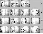 |
While a formal study has not yet been performed, an estimate of performance can be postulated. It has been shown that the algorithm is extremely general, based on the stated formation classification, as well as the promise in future work to expand the list of formations attainable. Results in Tables (2 & 4) show that a formation remains stable once it has been established (note that Equation 11 guarantees relationship stability). The algorithm is independent of the number of robots and is, thus, robust to group size; this can be actively demonstrated once a dynamic neighborhood method has been implemented. As seen in 1-dimensional Robot-Space Cellular Automata, an operator can quickly and easily manipulate a formation in a variety of different ways.
Formation management
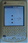
In multi-robot management, little work has been done in terms of a human-robot interface for formations. Skubic et al. [26] implemented an impressive sketch-based interface via Personal Digital Assistant and global communication to control a small team of mobile robots already in formation [Fig. 39]. This proves to be inadequate for SSP, and thus an original interface must be designed and created for the control of large robotic formations.
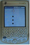  |
To manage the robot formation, a graphical user interface could be developed that would provide a human operator with a visualization of the formation and information of each individual robot unit. Through the interface, the operator would be able to choose the seed robot to instigate a change in the formation.
Multi-robot sandbox
The robot platform presented provides a variety of tools that can be used to implement and test various multi-robot systems. While homogeneous in terms of hardware, unique physical identifiers combined with addressed communication allow for heterogeneous applications. To keep with a theme of this work, consider a physical implementation the most well-known example of cellular automata, Conway’s Game of Life [29]. To be consistent, let The Game be represented as a Class I swarm in a 2-dimensional robot-space cellular automaton (note that this could also be represented in world-space). A cell neighborhood could consist of all cells within the automaton, with relationships—and not the cells themselves—in a state of “alive” or “dead”; strict rules, based on the states of these relationships, would dictate robot actions, producing interesting emergent behavior. The platform serves as a “sandbox” for multi-robot creativity—the possibilities are endless.
Publications and Recognition
This work has received considerable attention in the academic and professional communities, warranting publications, presentations, grants, and awards.
Proceedings
2011
- Beer, B., Mead, R., and Weinberg, J.B. (2011) A Distributed Spanning Tree Method for Extracting System and Environmental Information from a Network of Mobile Robots. In The 2011 Association for the Advancement of Artificial Intelligence Spring Symposium on Multi-Robot Systems and Physical Data Structures (SS-11-07), Stanford, California. [PDF]
- Mead, R. and Kaszubski, E. (2011) A Distributed Multi-Layered Cellular Automata Approach to the Hierarchical Structural Organization of Multi-Robot Systems. Submitted to The 2011 Association for the Advancement of Artificial Intelligence Spring Symposium on Multi-Robot Systems and Physical Data Structures (SS-11-07), Stanford, California. [PDF]
2010
- Beer, B., Mead, R., and Weinberg, J.B. (2010) A Distributed Method for Evaluating Properties of a Robot Formation. In the Student Abstract and Poster Program of the 24th AAAI Conference on Artificial Intelligence (AAAI 2010), Atlanta, Georgia. [PDF]
2009
- Mead, R., Long, R., and Weinberg, J.B. (2009). Fault-Tolerant Formations of Mobile Robots. In the Proceedings of The 2009 IEEE/RSJ International Conference on Intelligent Robots and Systems (IROS-09), 4805-4810, St. Louis, Missouri. [PDF] [PPT]
2008
- Mead, R. and Weinberg, J.B. (2008). A Distributed Control Algorithm for Robots in Grid Formations. In the Technical Report (WS-08-02) of The 2008 Association for the Advancement of Artificial Intelligence (AAAI-08) Workshop on Mobile Robotics: Mobility and Manipulation, Chicago, Illinois. [PDF]
- Mead, R. and Weinberg, J.B. (2008). 2-Dimensional Cellular Automata Approach for Robot Grid Formations. In the Student Abstract and Poster Program of the 23rd National Conference on Artificial Intelligence (AAAI-08), 1818-1819, Chicago, Illinois. [PDF] [Poster]
- Weinberg, J.B. and Mead, R. (2008). A Single- and Multi-Dimensional Cellular Automata Approach to Robot Formation Control. Submitted to The 2008 IEEE International Conference on Robotics and Automation (ICRA-08), Pasadena, California. [PDF]
2007
- Mead, R., Weinberg, J.B., and Croxell, J.R. (2007). A Demonstration of a Robot Formation Control Algorithm and Platform. In the Proceedings of the Robot Competition and Exhibition of the 22nd National Conference on Artificial Intelligence (WS-07-15), 23-27, Vancouver, British Columbia. [PDF]
- Mead, R., Weinberg, J.B., and Croxell, J.R. (2007). An Implementation of Robot Formations using Local Interactions. In the Proceedings of The 22nd National Conference on Artificial Intelligence (AAAI-07), 1889-1890, Vancouver, British Columbia. [PDF] [PPT]
2006
- Mead, R. and Weinberg, J.B. (2006). Algorithms for Control and Interaction of Large Formations of Robots. In the Student Abstracts and Poster Program of the 21st National Conference on Artificial Intelligence (AAAI-06), 1891-1892, Boston, Massachusetts. [PDF] [Poster]
Presentations
2011
- Choi, C., O'Hollaren, J., Mead, R., and Matarić, M.J. (2010). A Distributed Thermodynamics-Inspired Approach to Multi-Robot Obstacle Avoidance. Presented at the 13th Annual USC Undergraduate Symposium for Scholarly and Creative Work. Los Angeles, California. [Poster]
2008
- Mead, R. and Weinberg, J.B. (2008). Simple Cellular Automata Produce Complex Robot Grid Formations. Presented at The 2008 SIUE Graduate Student Research Symposium. Edwardsville, Illinois.
2007
- Mead, R., Weinberg, J.B., and Croxell, J.R. (2007). An Implementation of Robot Formations using Local Interactions. Presented at the Robot Competition and Exhibition of the 22nd National Conference on Artificial Intelligence (AAAI-07), Vancouver, British Columbia. [PDF] [PPT]
- Mead, R. and Weinberg, J.B. (2007). A Platform for Local Interactions between Robots in Large Formations. Presented at The 2007 SIUE Senior Project Showcase. Edwardsville, Illinois.
- Mead, R. and Weinberg, J.B. (2007). Algorithms for Control and Interaction of Large Formations of Robots. Presented at The 2007 SIUE Graduate Student Research Symposium. Edwardsville, Illinois. (SIUE Best Poster Award).
2006
- Mead, R. and Weinberg, J.B. (2006). Algorithms for Control and Interaction of Large Formations of Robots. Presented at the Student Abstracts and Poster Program of the 21st National Conference on Artificial Intelligence (AAAI-06). Boston, Massachusetts. [PDF] [Poster]
- Mead, R., Weinberg, J.B., and White, W. (2006). Algorithms for Control and Interaction of Large Formations of Robots. Presented at The 2005-2006 SIUE Undergraduate Research Academy Symposium. Edwardsville, Illinois.
- Mead, R., Weinberg, J.B., and White, W. (2006). Algorithms for Control and Interaction of Large Formations of Robots. Presented at The 2006 SIUE Graduate Research Symposium. Edwardsville, Illinois.
Theses
2010
- Long, R. (2010). Distributed Auction-Based Initialization of Mobile Robot Formations. Master's Thesis, Southern Illinois University Edwardsville. [PDF]
2008
- Mead, R. (2008). Cellular Automata for Control and Interactions of Robots in Large Formations. Master's Thesis, Southern Illinois University Edwardsville. [PDF] [PPT]
Grants
2010
- Mead, R., Choi, C., O'Hollaren, J., and Matarić, M.J. (2010). A Distributed Approach to Multi-Robot Obstacle Avoidance. Principal Investigator. Funded by 2010-2011 University of Southern California Undergraduate Research Associates Program. ($6600). Completed 2011.
2007
- Mead, R. (2007). Cellular Automata for Control and Interaction of Large Formations of Robots. Principal Investigator. Funded by Fall 2007 Research Grants for Graduate Students Award. ($330). Completed 2008.
2005
- Mead, R., Weinberg, J.B., and White, W. (2005). Algorithms for Control and Interaction of Large Formations of Robots. Principal Investigator. Funded by 2005-2006 Undergraduate Research Academy Award. ($1200). Completed 2006.
Awards
2007
- Technical Innovation Award for Multi-Robot Coordination. (2007). Awarded by the Robot Competition and Exhibition of the 22nd National Conference on Artificial Intelligence (AAAI-07). Vancouver, British Columbia.
- SIUE Best Poster. (2007). Awarded by The 2007 SIUE Graduate Student Research Symposium. Edwardsville, Illinois.
2005
- SIUE Undergraduate Research Academy Scholar. (2005). Awarded by the 2005-2006 SIUE Undergraduate Research Academy. Edwardsville, Illinois.
