1-Dimensional Robot-Space Cellular Automata
In Mead et al. [19, 20], each robot is represented as a cell ci in a 1-dimensional robot-space cellular automaton, where i refers to the index within the automaton; note that an index is not necessarily the robot’s identification number or address that is used for communication—it is simply a reference. A cell consists of a neighborhood H, a state s, a formation definition F, and a step function S (each of these variable concepts will be described in detail throughout this chapter), written as:
Neighborhood
Each cell ci is part of a neighborhood Hi, where:
Cells ci-1 and ci+1 refer to the left and right neighbors of ci within the automaton, respectively. Likewise, a particular neighbor is denoted cj, where j is the index of the cell representing a neighboring robot. It follows that, by combining the neighborhoods of all n cells, connectivity is enforced when defining the entire automaton C:
State
The state si of a cell ci consists of the following variables: p, the relative position of the cell within the formation (referred to as formation-relative position); rdes, the set of all desired relationships with neighboring cells; ract, the set of all actual relationships with neighboring cells; Θ, the rotational error of the robot within the formation; Γ, the translational error of the robot within the formation; t, the time step of the cell (each of these variable concepts will be described in detail throughout this chapter). Formally:
In cellular automata, to determine the state sit of ci at time t, it must consider the state of all cells in Hi at the previous time step. A state transition step function—or step function—S (see State Transition for details on how this determines the state) can be written such that:
Formation Definition
A desired formation F is defined by: f(x), a geometric description (in this chapter, a single mathematical function); R, the desired distance to maintain between neighbors in the formation; Φ, the orientation of each robot relative to the formation on an x-/y-coordinate system (referred to as formation-relative orientation); pseed, a formation-relative position that serves as a starting point from which the formation and relationships will propagate.
This definition is sent to some robot, designating it as the seed cell cseed of the automaton. Note that cseed is not a leader, but rather an initiator of the coordination process.
State Transition
For purposes of establishing neighborhood relationships, a cell considers itself to be at some formation-relative position pi (in the case of cseed, pseed is given in F):
Relationships
Desired relationships
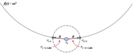
. Relationships are determined by calculating a vector v from pi to the intersection of f(vx) and a circle centered at pi with radius R (given in F):
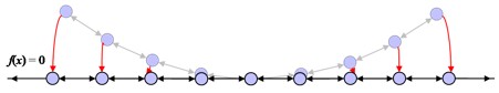
Solving for the desired relationship vector ri→j,des to some neighbor cj results in two intersections: one in the positive direction and one in the negative direction. These solutions define right and left neighbor relationships ri→i+1,des and ri→i-1,des, respectively; these relationship vectors are then rotated by –Φ, the negation of the given formation-relative orientation, so that robot heading is consistent within the formation definition [Fig. 15].
 |
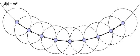
The formation definition and relationship information are communicated locally within the Hi. Neighboring robots repeat the process, but consider themselves to be at different formation-relative positions as determined by the desired relationship from their neighbor. For a neighbor cj:
Note that relationships rj→i,des and ri→j,des are equal in magnitude, but opposite in direction. This property of the algorithm is what guarantees convergence and stability between two robots attempting to establish and maintain relationships with one another. These calculated desired relationships generate a connected graph that yields the shape of the formation [Fig. 16].
 |
Actual relationships
. Using only sensor readings, robots calculate an actual relationship ri→j,act with a neighbor cj (see Robot Platform for details on how this relationship is determined). The robot communicates locally (i.e., within the neighborhood) discrepancies in its desired and actual relationships to neighboring cells. Correcting for these discrepancies produces a robot movement action Ai (discussed below) for each ci, resulting in the overall organization of the desired global structure.
Motion control
By evaluating the state of the Hi, ci is able to determine the translational error Γi and rotational error Θi (a difference from actual to desired) that will define its movement action Ai in the physical world:
(For simplicity, Ai is assumed to be along a safe trajectory.)
To determine values for Γi and Θi, ci must first seek a point of reference. Recall that the seed cell cseed was given an initial formation-relative position pseed, from which the formation and relationships propagate. As the distance from cseed increases, the propagated error accumulates. It follows that the neighbor of ci whose formation-relative position is closest to pseed will have the least amount of propagated error within the system and, thus, will likely represent the most reliable robot to reference. This reference neighbor ck is then the neighbor that yields the minimum distance ||pk′|| from pseed to pk:
Rotational error
. The rotational error Θi is a difference in robot orientation, which is propagated to each successive cell in the automaton. To determine Θi, ci considers rk→i,act with respect to itself. Let θi→k represent the relative angle between the headings of ci and ck, and let θi and θk be the angles of the relationship vectors ri→k,act and rk→i,act, respectively. Then:
Note that when θi→k = 0°, both i and k have the same global heading. The same holds true for every robot in the formation if Θi = 0° for all i. This property of the algorithm to yield an emergent global heading is essential for any subsequent teleoperation from an operator. If a translational movement command is given, the common heading of the robots allows for a smooth transition in the same direction.
Translational error
. The appropriate translational movement for each robot represented in the automaton is determined by an accumulation of error with both x- and y-components. This error is determined by the difference in desired and actual relationships of reference cell ck. One major consideration is that many of the robots are, themselves, correcting for translational and rotational errors while they are being referenced by other robots. Changes in the orientation of ck can cause rather entropic behavior in ci, which depends on it for motion control. To alleviate this problem, rk→i,des must be rotated, accounting for the propagated rotational error Θk within the automaton. Let rk→i,des′ denote rk→i,des rotated by an angle –Θk; γi can be expressed as the translational error of ci with respect to ck:
The Γk term represents the accumulation of error from ck. Recall that θi→k relates the headings of both of these robots, providing a conversion between the relative coordinate systems of ci and ck. Thus, rotating γi by –θi→k yields the translational error Γi.
Formation Manipulation
To show the dynamic switching capabilities of the algorithm, a human operator can send a variety of commands to the seed cell, thus, propagating changes in the automaton and causing a chain reaction in neighboring cells, which then change states accordingly, resulting in a global transformation of the formation.
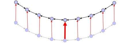
Formation translation
A translation command Ψ (with both x- and y- components) moves the robots relative to the current formation-relative orientation Φ. [Fig 17]. This is done by “tricking” the cells and taking advantage of the motion control system as defined above; simply add Ψ to the current translational error of the seed, and the error will be propagated:
 |
Formation rotation
A formation rotation command Ω causes a change in the orientation of the formation as a whole, thus, requiring each robot to move in such a way as to maintain the shape as it is rotated [Fig. 18]. Taking advantage, again, of the motion control system, the rotational error of the seed Θseed is simply rotated by Ω:
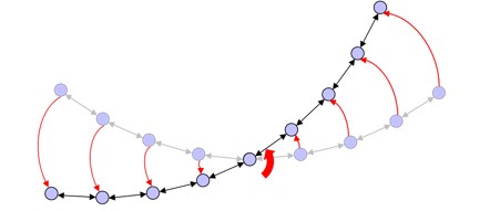 |
Cell rotation
A cell rotation command φ modifies the orientation of each cell relative to the formation; this contrasts to the formation rotation command in that the position and orientation of the formation itself relative to an external frame of reference remain unchanged [Fig. 19]. To do this, the seed cell prepares to perform a rotation in a similar way to that of a formation rotation command; it rotates Θseed by φ. To prevent the entire formation from moving, it also rotates the formation-relative orientation Φ by this amount in the opposite direction and recalculates its desired relationships; this instigates a change in relationships through all cells in the automaton:
 |
Formation scaling
A scaling command z stretches each of the desired relationships of ci by the given scalar [Fig. 20]. For every neighbor cj:
 |
Formation resizing
A resizing command Z multiplies R (the distance that neighboring robots should stay apart) by this factor [Fig. 21]. This command is similar to the scaling command, but differs in that desired relationships must actually be recalculated using Equations 8 & 9 instead of being directly manipulated by some scalar:
 |
Formation change
To change a formation, a seed cell is chosen and given the new geometric description, and the process described above is repeated [Fig. 22].
 |
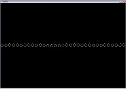
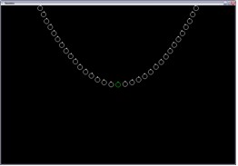
Simulator
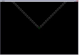
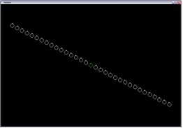
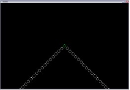
The control algorithm was initially implemented in a simulated environment [19; Simulator Code]. The simulator was written in C++ using OpenGL, and provides an easy means to visualize, manipulate, and test the algorithm; an operator may directly manipulate any cell, relocating or reorienting it to evaluate the stability of the system in the presence of error [Fig. 23].
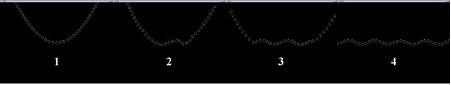 |
As before, each robot is represented as a cell ci, where i is the corresponding index within the automaton; in the simulator, the automaton is stored as a 1-dimensional array of n cells, where n is given at runtime. Tens-to-thousands of cells have been tested against various formation definitions to demonstrate the scalability and generality of the algorithm [Table 1].
 |
f(x) = 0 |
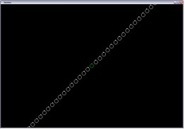 |
f(x) = x |
 |
f(x) = |x| |
 |
f(x) = –½ x |
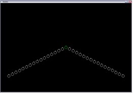 |
f(x) = –½ |x| |
 |
f(x) = –|x| |
 |
f(x) = x2 |
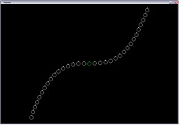 |
f(x) = x3 |
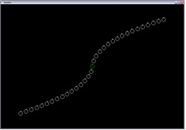 |
f(x) = {–√|x|, if x < 0 | else, √x} |
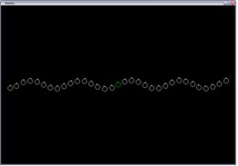 |
f(x) = 0.05 sin(10 x) |
| (Note that, for all formations shown here, R = 10.5", Φ = 90.0°, pseed = [ 0.0 0.0 ]T.) | |
The simulator makes several simplifying assumptions. First, the array of cells is updated in discrete and synchronized time intervals; this alleviates any problems of inconsistency within the automaton. Second, each neighborhood has already been established; for a cell at index i, this neighborhood consists of the cells at the left and right indexes i-1 and i+1, respectively. Finally, each cell is assumed to have perfect, continuous, and unlimited sensing; thus, a cell is able to get its distance and orientation to any other cell at any point in time.
The next section discusses the physical implementation of this algorithm and how these assumptions were overcome to prove that the approach is viable in the real world.
Robot Platform
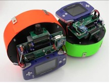
A platform was developed to test the algorithm in the physical world [20; Fig. 24]. Each robot is built upon a Scooterbot II base [www.budgetrobotics.com]. The Scooterbot is 7 inches in diameter and is crafted from expanded PVC, making it durable and light. Two modified servo motors are employed for differential steering.
 |
Controller
The formation control algorithm is implemented in Interactive C (IC) [www.botball.org/ic] and runs on an XBCv2 microcontroller [Fig. 25; www.botball.org]. The XBC utilizes back-EMF PID for accurate motor control. It also features a camera, capable of multi-color, multi-blob simultaneous tracking. Rotating the robot provides a 360° view of the environment and neighboring robots.
 |
Neighbor localization
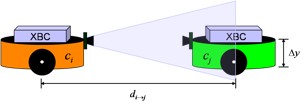
A neighboring robot represented by cj is identified by either an orange or green color band; the color of each robot is assigned based on its ID: green for even; orange for odd. The alternating of color bands reduces the chances of overlapping color blobs and improves the accuracy of detecting a neighbor.
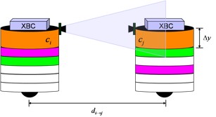
Relative distance
. To locate cj, a robot represented by ci rotates until the band of the appropriate color is within its view; it then centers on that band. The heading of ci is always considered to be directed at the x-axis (0°); relative to the robot, left yields positive angles and right yields negative angles. The distance di→j between ci and cj is determined by recognizing that the perceived vertical displacement Δy between the top and bottom of a color band is proportional to the perceived vertical displacement ΔY at a known physical distance D [Fig. 26]:
 |
Relative orientation
. The relative orientation αi→j from ci to cj is simply the angular displacement from the initial location (i.e., prior to the search) of ci. Thus, the actual relationship vector ri→j,act is written in polar coordinates as:
Communication
Hardware
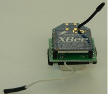
. A radio communication module is used to share formation and state information within a robot’s neighborhood. The Digi XBee (ZigBee/IEEE 802.15.4 compliant) was chosen for its rich feature set [www.digi.com]. The module does not require a host/slave configuration, allowing for mesh networking and packet rerouting. The XBee also scales well for large applications, using 16-bit addressing to provide for over 65,000 nodes. The low-power model offers a range of 100 meters, which is equivalent to class-2 Bluetooth. The chip communicates using a TTL-level UART, while the XBC uses RS-232 levels. A PCB was designed by J.R. Croxell [20] to overcome level translation and to interface between the XBee and the XBC. All parts are surface mounted, with the exception of a 9-pin D-Sub male plug. The result is a board smaller than the XBee itself that directly plugs into the XBC’s 9-pin serial port [Fig. 27].
 |
Software
. Digi offers a wide range of functionality and extensive documentation for the XBee [29]; this eased the implementation and integration of a reliable packet communication system, supporting automatic retries and acknowledgments. The communication library developed allows values of different types to easily be “packed” (queued) into a buffer for sending and “unpacked” (dequeued) from a buffer when receiving (see Communication.ic in Robot Code for details). Packets can be addressed to a particular robot or broadcast. This allows each robot to communicate locally within its neighborhood, relaying and querying formation and state information.
Behaviors
The simulator made the simplifying assumption of robots updating and moving in synchronous discrete time steps. However, in the real world, one must consider that each robot will be updating and moving in asynchronous continuous time. This problem is alleviated by using a finite state representation to safely transition between a series of behaviors, while maintaining an internal counter (time step independent of system clock) of events (state updates) that have occurred [Fig. 28]. This preserves the concept of discrete time in classic cellular automata.
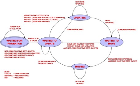 |
WAITING FOR FORMATION
. This is the initial (entry-point) behavior of the robot. The robot will wait indefinitely until it receives a formation definition from either the operator (designating it as the seed cell in the automaton) or from a neighboring robot (queried at robot startup and/or relayed upon receiving a formation definition itself).
WAITING TO UPDATE
. The robot must make certain that its neighbors are not moving or preparing to move before it updates its state, as a moving robot would make determining an instantaneous actual relationship impossible. This behavior also functions as a checkpoint for synchronizing the current time step t of a cell within its neighborhood; the entire neighborhood is synchronized when all time steps are equal. To synchronize, the time step ti of the cell ci is set equal to the maximum of all neighborhood time steps:
This is particularly useful when introducing a new robot into the formation. At startup, its neighborhood is queried for a formation definition and, subsequently, the time step. With this information, a cell can seamlessly enter into the automaton.
UPDATING
. During the update process, the robot determines its actual relationship to each neighbor within its neighborhood (see Neighbor localization above for how this relationship is determined). The robot then calculates its translational and rotational error, increments its time step ti, and finally communicates its new state sit locally within its neighborhood.
WAITING TO MOVE
. This behavior is similar to the WAITING TO UPDATE behavior; the robot must wait until all neighbors are done updating before moving. Once all neighbors are done updating, their time steps should all be synchronized. If an inconsistency occurs, the robot reports an error and returns to the WAITING TO UPDATE state for synchronization.
MOVING
. While executing this behavior, the robot actually attempts to correct for its calculated error, translating and rotating based on its movement action Ai. Upon completion, the translational and rotational error are approximately 0, and the state is updated to reflect this; the time step ti is incremented for this state change, and the state sit is communicated to the neighbors of the cell.
Implementation Results
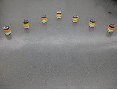
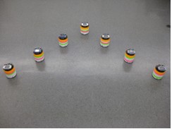
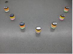
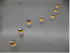
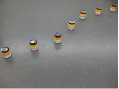
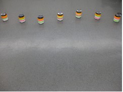
The algorithm was implemented on a variety of different formation using twelve of these robots (shown below in different numbers with different identification bands, as these pictures were taken during the process of this thesis; see Neighbor Identification in the next section for how these robots are identified).
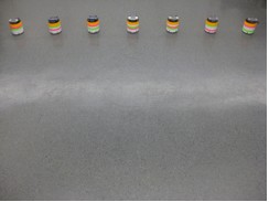 |
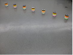
f(x) = 0 |
 |
f(x) = x |
 |
f(x) = |x| |
 |
f(x) = –½ x |
 |
f(x) = –½ |x| |
 |
f(x) = –|x| |
 |
f(x) = 1/64 x2 (16.0" focus) |
 |
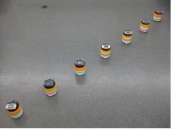
f(x) = (0.1 x)3 |
 |
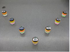
f(x) = {–5 √|x|, if x < 0 | else, 5 √x} |
 |
f(x) = 8 sin(3 x) |
| (Note that, for all formations shown here, R = 24.0", Φ = 90.0°, pseed = [ 0.0 0.0 ]T. Also, the perspective of the camera was changed to keep seven robots in the image.) |
|
2-Dimensional Robot-Space Cellular Automata
Goals and Objectives
Extending the formation control algorithm to be applied to SSP, the global structure of the solar reflector array could be viewed as a 2-dimensional lattice of robots. In [10, 11, 19, 20, 28], the formations were setup so each robot only needed to identify two neighbors. In the reflector formation, the definition of a neighborhood becomes more complex. There are various neighborhoods defined for cellular automata, such as the von Neumann Neighborhood (four surrounding cells), Moore Neighborhood (eight surrounding cells), and the Extended Moore Neighborhood (includes cells adjoining the immediate eight surrounding cells) [23]. Landis [15] provides insight into potential physical configurations of robots for SSP and this is considered in determining the appropriate number of neighbors for a given formation [Fig. 29]. The proper neighborhood definition for the automaton is crucial because it will directly affect how each robot cell reacts, how information gets propagated through the formation, and influences the overall performance of the formation by increasing or decreasing the communication and sensing overhead.
Extending the Formation Definition
Mead et al. [19] identified the potential for different categorizations of formations (see Formation classification in the Conclusions for a preliminary analysis), including those that are defined by multiple functions. To do so, the initial formation definition F must be extended to include more than one function. Let f' be a set of M mathematical functions used to define the shape of the formation, such that F in Equation 6 can be extended:
Each function is considered individually for purposes of calculating desired relationships and, thus, generates its own 1-dimensional neighborhood as before; this results in M neighborhoods. To extend Equation 2, consider a neighborhood mhi for a single function fm(x), where 1 ≤ m ≤ M:
The combined neighborhood can then be represented as the union of all M neighborhoods:
Note that ci is unique within the automaton as a whole and is a common intersection of each neighborhood for each function; to illustrate this, Hi can be expanded:
Similar to its previous definition, any particular neighbor can be written as mcj, where m refers to the function upon which j is an index to a neighboring cell. It follows that the step function S must also consider the new neighborhood for purposes of calculating the state sit:
This distinction is especially important f determining the aforementioned reference neighbor ck; extending Equation 13 to consider all neighbors within a neighborhood defined by multiple functions, the identity of ck can still be determined. The reference neighbor ck can be defined, similar to before, as the neighbor that with the minimum distance ||pk'|| from pseed to mpk, where m refers to the function upon which k is the index to the cell to be referenced:
| k | pk′ = min({||Mpi-1 – pseed||, ..., ||2pi-1 – pseed||, ||1pi-1 – pseed||, ||1pi+1 – pseed||, ||2pi+1 – pseed||, ..., ||Mpi+1 – pseed||}) | (Eq. 32) |
Formations Defined by Multiple Functions
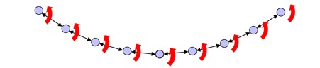
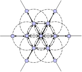
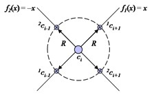
As an example and for purposes of SSP [15], consider a hexagonal lattice structure by defining a formation F by three functions: f1(x) = 0, f2(x) = x √3, and f3(x) = –x √3. For cseed, solving for Equations 8 and 9 for each of these functions yields a total of six desired relationships [Fig. 30].
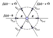 |
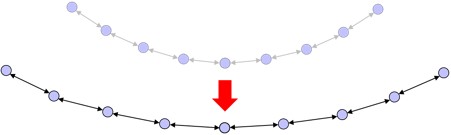
As before, the definition and relationships are propagated to neighboring cells, which repeat the process. However, using the standard implementation of the algorithm, the resulting formation would be a sort of “six-armed structure” [Fig. 31].
 |
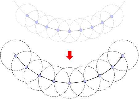
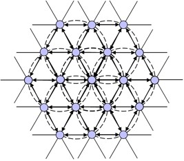
The formation of this structure is the product of the pi term in Equation 8, which considers the cell ci to be at position pi on some function and, in turn, affects the calculation of desired relationships in Equation 9. While this may be desirable for some applications, it deviates from the goal of a lattice. By removing the pi term from Equation 8, all cells will be considered at the origin when calculating their desired relationships on all M functions:
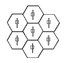
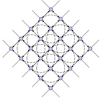
Note that the pi term does not leave the algorithm completely—it is still propagated within the automaton for purposes of determining the reference neighbor in Equation 31. This seemingly minor change produces significant results: cells begin to develop common neighbors as neighborhoods intersect one another; an emergent hexagonal lattice structure results [Fig. 32].
 |
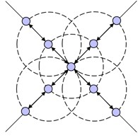
Now, consider using the functions f1(x) = x and f2(x) = –x to define F in order to generate a square lattice [Fig. 33].
 |
Similarly to that of the hexagonal lattice attempt, if the standard implementation is used, a “four-armed structure” results that was not intended (but nonetheless interesting) [Fig. 34].
 |
However, as before, by utilizing Equation 33 for purposes of determining desired relationships, the desired lattice forms from this multi-function definition [Fig. 35].
 |
Neighbor Identification
For a robot to determine its state, it must be able to identify its neighbors. This is easier said than done, as each unit looks identical. The problem is analogous to being in a room of people that look and dress exactly alike; if one person speaks (i.e., sends a message) without further sensory input, such as auditory localization, it is impossible to determine who was speaking. A colored bar-coding system is utilized to alleviate this problem; each robot features a unique “face”—a three-color column, where the vertical locations of the green and magenta bands (in relation to the orange band) correspond to its identification number [Fig. 36].
 |
Relative distances are calculated as in Equation 22 using only the orange color bar at the top. However, for an orange band in a camera frame to even be considered a neighboring robot, it now must also possess a green band and a magenta band at some nearby position beneath it; based on the proportions of the size of these bands in the physical world, it is simple to tell whether or not a perceived combination of bands in a frame is valid. The identification number of the robot is determined based on the following table (note that, when the green band is above the magenta band, this number is even and vice versa):
 |
0 |  |
1 | |
 |
2 |  |
3 | |
 |
4 |  |
5 | |
 |
6 |  |
7 | |
 |
8 |  |
9 | |
 |
10 |  |
11 | |
 |
12 |  |
13 | |
 |
14 |  |
15 | |
 |
16 |  |
17 | |
 |
18 |  |
19 |
While a greater number of robots could have been identified using all permutations of color combinations, requiring that all three color bands be present and that one be in a fixed position simplifies vision processing, while still providing enough unique identifiers for the number of robots implemented.
Implementation Results
This extension of the algorithm was implemented and tested on 19 “face-lifted” robots (shown below in different numbers) [Table 4]. Integration with the previous implementation was seamless, as relationships are calculated for any number of functions. A flag is set to specify whether Equation 8 or Equation 33 is to be used.
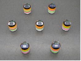 |
f1(x) = 0
f2(x) = x √3 f3(x) = –x √3 R = 24.0" Φ = 90.0° pseed = [ 0.0 0.0 ]T |
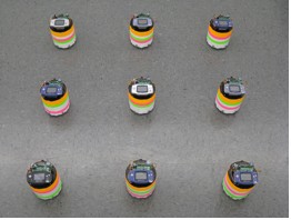 |
f1(x) = x
f2(x) = –x R = 24.0" Φ = 45.0° pseed = [ 0.0 0.0 ]T |
